How to Estimate Dilution Effects in Experiment and When to Ignore it

Jinqi Shen

Summary

Dilution effects in A/B testing refer to the scenario where unrelated traffic is included in the experiment, thereby reducing its efficiency. Although this phenomenon is widely recognized in the industry, there is a lack of quantitative analysis—at least in common blogs, discussions, or mature packages—regarding the extent of its impact. This blog aims to address this gap by offering insights into when this issue requires careful attention and when it can be safely disregarded.

Given this blog will be relatively lengthy and complex in math, I would like to provide an overview of the main result:

This blog introduces a scientific formula, complemented by Python code, to quantify the efficiency loss caused by the dilution effect. Using this formula, experiment designers can assess the efficiency reduction and make well-informed decisions about whether to adopt stricter triggering mechanisms.
In general, a higher dilution proportion results in lower efficiency. However, there are specific scenarios where efficiency remains high even with a significant dilution proportion. This tends to occur when the dilution proportion is reporting a constant value, and the means of the treatment and control groups are close to this constant value.
Eliminating unrelated traffic either prior to or following the experiment can completely mitigate the dilution effect and we will discuss in details later.

Problem Statement

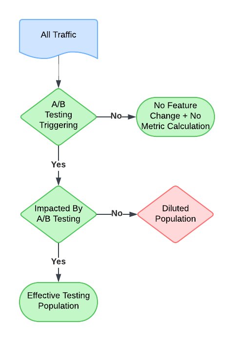
As previously mentioned, the dilution effect occurs when unrelated traffic is included in the experiment, introducing additional and unnecessary noise into metric calculations and reducing the overall efficiency of the experiment.

The diagram below illustrates this concept. The dilution specifically corresponds to the red portion, which represents instances triggered by the experiment and reported in the metrics but are not actually affected by the experiment.

It is commonly understood in the data science industry that including diluted traffic reduces the efficiency of experiments. Ideally, experiment triggering should be as closely aligned with the actual change as possible to minimize the diluted proportion. However, this ideal scenario is not always feasible in practice. Various constraints, such as technical limitations, data availability, or operational complexity, may prevent the perfect alignment of triggers with changes:

It can be due to engineering complexity but whether the user is related to the experiment can be logged.
- Consider the example of testing a drop-down menu on a web page. The experiment is triggered when the user requests the page, but it is unclear whether the user will interact with the drop-down. In this case, users who request the page but do not interact with the drop-down become part of the diluted population.
- To address this, interactions with the page component can be logged and used to adjust for the dilution effect. This approach, which will be discussed in greater detail later, provides a practical way to mitigate the impact of unrelated traffic on experiment efficiency.
In some cases, dilution effects arise due to unobserved latent variables, making it impossible to log whether traffic is related to the experiment.
- For example, click-through rate (CTR) is a critical metric for measuring ad performance. However, some users exposed to the experiment may constitute a diluted population because their response to the ads is either nonexistent or undetectable. This could occur if:
  - They use ad blockers that cannot be detected.
  - The ads are entirely irrelevant to them, such as a renter viewing ads for mortgage refinancing.
  - In such scenarios, the dilution effect is challenging to address directly, but understanding these limitations is crucial for interpreting experimental results and designing more effective experiments.

In both cases above, the dilution effect has a significant impact on the experiment. However, as we will explore later, the existence of logging allows us to almost completely eliminate the dilution effect in the first case. Unfortunately, in the second case, due to the presence of unobserved latent variables, the dilution effect cannot be fully removed.

In addition to the classifications above, experiments with dilution can also be divided into the following two scenarios:

The diluted part always reports a constant. For instance, in the ads example discussed earlier, users in the diluted population always exhibit no response to the ads. This scenario represents a predictable and consistent dilution effect.
The diluted part reports non-constant values. For example, in an experiment on a hotel booking website aimed at measuring the number of bookings, users in the diluted population can still make bookings even if they are irrelevant to the experiment. This scenario introduces variability into the dilution effect, making it harder to quantify and address.

Understanding these scenarios is crucial for developing tailored strategies to mitigate the dilution effect and improve experiment efficiency.

Quantitative Analysis on Dilution Effect

Now we come to the exciting and complex part, which is the quantitative analysis. Please follow carefully as we begin by defining certain mathematical notations that will be used throughout the document.

Notations

Assume we are comparing two groups, treatment and control (the conclusion in this document can be easily generalized to the situation of having more than two groups). Assume the populations for treatment and control groups are $X_T$ and $X_C$ respectively, and they have expectation and variance being $(\mu_T,\sigma^2_T)$ and $(\mu_C,\sigma^2_C)$ . We are interested in comparing if there are differences between $\mu_T$ and $\mu_C$ .

In the classic experiment setting, in both groups, we will observe independent samples ${X_{C,i}}_{i=1}^{n_C}$ and ${X_{T,i}}_{i=1}^{n_T}$ , where $n_C$ and $n_T$ are sample sizes of the control and treatment groups, and leverage the sample mean difference as the test statistics, which is $\Delta = \bar{X}_C - \bar{X}_T$ . Under some mild conditions, $\Delta$ has an approximate distribution $\Delta\sim N(\mu_C -\mu_T, \sigma^2_C/n_C + \sigma^2_T/n_T)$ . Apparently, the detection probability is only related to the ratio between the absolute mean difference and standard deviation, which is $\frac{|\mu_C-\mu_T|}{\sqrt{\sigma^2_C/n_C + \sigma^2_T/n_T}}$ .

Now, under a diluted experiment setting, we only can observe $X_C$ and $X_T$ with some probabilities. Statistically, we can only observe $\{X'_{C,i}\}_{i=1}^{N_C}$ and $\{X'_{T,i}\}_{i=1}^{N_T}$ , where $X'_{C,i} = X_{C,i} I_{C,i} + Z_{C,i}(1-I_{C,i})$ , $X'_{T,i} = X_{T,i} I_{T,i} + Z_{T,i}(1-I_{T,i})$ , ${I_{C,i}}$ and ${I_{T,i}}$ both independently follow the same Bernoulli distribution $B(0,1)$ with probability $p$ , and ${Z_{C,i}}$ and ${Z_{T,i}}$ both independently follow the same distribution $Z$ with mean $\mu_Z$ and variance $\sigma_Z^2$ . To avoid confusion, we use the distribution of $Z$ to indicate the diluted part distribution and $p$ being the probability that the triggered cases in the diluted experiment is related to this experiment. And roughly we have $n_C = p N_C, n_T = p N_T$ .

Then with the diluted data, the corresponding test statistics is $\Delta':=\bar{X}'_C - \bar{X}'_T$ . Now, we want to know the mean and variance of this statistics. In addition to that, we want to know how much efficiency we are losing due to this diluted effect. In order to measure it quantitatively, we define the efficiency to be $C_{eff} = \frac{n_C}{p*N_C}$ , where $n_C$ and $N_C$ will make $\Delta$ and $\Delta'$ have the same detection power. As for interpretation, we can say in order to achieve the same detection power, we need $1/C_{eff}$ times more samples (after the conversion rate of $p$ ).

Main Results and Discussions

The first result presented here is about the property of $\Delta'$

Result 1:

$\mathbb{E}[\Delta'] = p(\mu_C-\mu_T)$
$\text{Var}(\Delta') = \frac{1}{N_C}((\mu_C-\mu_Z)^2p(1-p)+(1-p)\sigma^2_Z+p\sigma^2_C) + \frac{1}{N_T}((\mu_T-\mu_Z)^2p(1-p)+(1-p)\sigma^2_Z+p\sigma^2_T)$
$C_{eff}=\frac{rp\sigma_C^2+p\sigma_T^2}{r((\mu_C-\mu_Z)^2p(1-p)+(1-p)\sigma^2_Z+p\sigma^2_C) + (\mu_T-\mu_Z)^2p(1-p)+(1-p)\sigma^2_Z+p\sigma^2_T}$ , where $r=n_T/n_C$ .

Remark 1:

Apparently, with $p\rightarrow 1$ , $C_{eff}\rightarrow 1$ . This aligns with our intuition that with less and less diluted traffic, we also lose less and less efficiency.
Assume $\sigma^2_Z>0$ and $p\rightarrow 0$ , then $C_{eff}\rightarrow 0$ . This means if the noise random variable is not a constant, then with more and more diluted traffic, we will eventually lose all detection power. This applies to the second situation that users in the diluted traffic contribute non-constant noise to the final result. In this case, dilution effect can be infinitely bad if there are too much diluted traffic.
Assume $\sigma^2_Z = 0$ and without loss of generality, assume $\mu_Z=0$ (since we can always subtract $\mu_Z$ from the distribution of treatment and control). Then with $p\rightarrow 0$ , $C_{eff}$ will also monotonically decrease, but it will converge to $C_{eff}=\frac{r\sigma_C^2+\sigma_T^2}{r(\mu_C^2+\sigma^2_C) + \mu_T^2+\sigma^2_T}$ . This applies to the first situation we have in the introduction where we are triggering samples from an early step in the funnel and those users who do not observe the difference will only contribute a constant to the final metric calculation. In this case, although dilution effect will still affect the experiment efficiency, it will not be infinitely bad. In fact, if the effort of moving the trigger is larger than the loss on the efficiency, we should do the trade off for it.
If the distribution on control and diluted part is the same (or very close) and $\sigma_C \approx \sigma_T$ and $\mu_C - \mu_T$ is small (compared to standard deviation), then we will have $C_{eff} \approx p$ , which is a very common cases in industry.
Some simple code for calculating $C_{eff}$ is provided in the Appendix.

From Result 1, we know that the diluted effect does exist, although the impact can be different under different scenarios. Now, the question is about whether we can have other solutions than just changing the triggering users logic.

Assume we can have additional information about the total number of users who could experience the difference designed in the experiment, i.e., we have $S_C = \sum_{i}I_{C,i}$ and $S_T = \sum_{i}I_{T,i}$ , then another intuitive test statistics would be $\widetilde\Delta':=\frac{\bar{X}'_{C}}{\bar{I}_C}-\frac{\bar{X}'_{T}}{\bar{I}_T}$ , where $\bar{I}_C=\bar{S}_C/N_C$ and $\bar{I}_T=\bar{S}_T/N_T$ (Intuitively, if $\sigma^2_Z = \mu_Z =0$ , this is just the sample mean after filter out unrelated users). Then how is the performance of $\widetilde\Delta':=\frac{\bar{X}'_{C}}{\bar{I}_C}-\frac{\bar{X}'_{T}}{\bar{I}_T}$ ?

Result 2:

With $n_C,n_T,N_C,N_T\rightarrow \infty,$

$\mathbb{E}[\widetilde\Delta'] \rightarrow \mu_C-\mu_T$
$\text{Var}(\widetilde\Delta') \rightarrow \frac{(1-p)\mu_Z^2+p(1-p)\sigma_Z^2+p^2\sigma^2_C}{N_Cp^3} + \frac{(1-p)\mu_Z^2+p(1-p)\sigma_Z^2+p^2\sigma^2_T}{N_Tp^3}$
If $\sigma^2_Z = \mu_Z =0$ , $C_{eff}\rightarrow 1.$

Remark 2:

Noticed that from claim 3 of Result 2, we will have the efficiency to be almost 1, which means asymptotically we will not lose any efficiency in detection.
Also, the setting of claim 3 is equivalent to marking all values from diluted population to 0, which requires the logging of actual impacted experiment elements.

Deep Dive into Special Cases

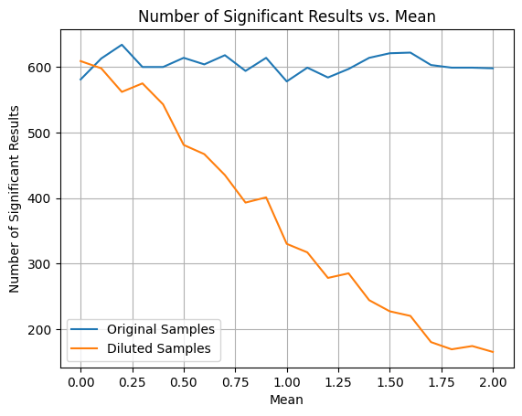
In general, there is not much surprising result with both results above, except for the one in the third point of Remark 1, where we concluded that when diluted population in the experiment always produce constant response, the diluted effect will converge to a constant when the dilution proportion converges to 1. Also, if means of treatment and control are not very different from that constant (relatively to standard deviation), the limit of the efficiency will be 1, means we can ignore the dilution effect.

This is in general counter intuitive as we commonly will think that with higher dilution proportion in the experiment, the detection power should converge to 0 as the noise will dominate.

We did the following simulations to validate the result above. Related code can be found here.

We generate two groups $X\sim N(\mu, 1)$ and $Y\sim N(\mu + 0.1, 1)$ , each with 1000 cases. We then diluted both groups by $p$ and fill in value 0’s. We then conduct T-tests for $X$ and $Y$ before and after diluted and check if the p-value is smaller than 0.05. We repeated this process for 1000 times and count how many times the related test will be significant.

We first fix $\mu = 1$ and varying $p$ to see if the efficiency will converge to a constant. The result is recorded in the table below. We can observe that with diminishing of $p$ , the number of significant results decrease but converges to roughly 338, which is supporting our result above.

Number of significant results within 1000 attempts vs varying diluted proportion $p$

We then fix $p = 0.1$ and observe those numbers with varying $\mu$ from 0 to 1. The result is recorded in the chart below. We can observe that the detection power will decrease with the increase of mean and when $\mu=0$ , the detection power is almost the same as the original sample, indicating we can ignore dilution effects in this case. And this also support our conclusion in theory.

Solutions for Resolving Dilution Effects

Now we come to the solutions for resolving dilution effects based on those insights from theory. Here are two ways that can almost fully resolve dilution effect:

Resolve during experiment triggering: totally remove / reduce diluted population from the experiment when the experiment is triggering.
Resolve after experiment triggering: keep a full logging of who actually experiences the difference in the experiment and only use them for analysis, or as indicated by Result 2 above, mark all other values to 0 for analysis.

Other than that, we can use the formula or function in the Appendix for calculation and understand if we can tolerate the information loss. If loss is small like those special cases mentioned above, we may save the effort for resolving the dilution effects as either solution mentioned just above may require extra engineer efforts.

Appendix

Note: The proof below is not fully rigorous, may need some mild conditions such that CLT and strong law will hold.

Proof for Result 1:

For Claim 1, $\mathbb{E}[\Delta'] = \mathbb{E}[X'_C]- \mathbb{E}[X'_T]=p\mu_C+(1-p)\mu_Z-p\mu_T-(1-p)\mu_Z=p(\mu_C-\mu_T)$

For Claim 2, by conditional variance, we have

$\text{Var}(X'_C) = \text{Var}(\mathbb{E}[X'_C|I_C]) + \mathbb{E}[\text{Var}(X'_C|I_C)]=(\mu_C-\mu_Z)^2p(1-p) + (1-p)\sigma_Z^2+p\sigma_C^2$

Similar result can be obtained for $\text{Var}(X'_T)$

Insert the formula into $\text{Var}(\Delta') = \text{Var}(\bar{X}_C) + \text{Var}(\bar{X}_T) = \text{Var}({X}_C)/N_C + \text{Var}({X}_T)/N_T$ , and we will obtain results in the Claim 2.

For Claim 3, simply let $n_C=C_{eff}N_Cp$ and solve $C_{eff}$ from $\frac{|\mu_C-\mu_T|}{\sqrt{\sigma^2_C/n_C + \sigma^2_T/n_T}}=\frac{p|\mu_C-\mu_T|}{\sqrt{\text{Var}(\Delta')}}$ .

Proof for Result 2:

For Claim 1, apparently $\bar{I}_C\overset{a.s.}\rightarrow p$ and therefore, $\mathbb{E}\big[\frac{\bar{X}'_{C}}{\bar{I}_C}\big]\rightarrow\mu_C+(1-p)/p\mu_Z$ (by Delta method). We can obtain similar result for $\mathbb{E}\big[\frac{\bar{X}'_{T}}{\bar{I}_T}\big]$ and the claim 1 is a direct result of it.

For Claim 2, we will first study $\text{Var}\big(\frac{\bar{X}'_{C}}{\bar{I}_C}\big)$ . By delta method, or simply Taylor expansion, we will have

$\text{Var}\big(\frac{\bar{X}'_{C}}{\bar{I}_C}\big) \rightarrow \frac{\text{Var}(X'_C)}{N_C(\mathbb{E}[I_C])^2}+\frac{\text{Var}(I_C)(\mathbb{E}[X'_C])^2}{N_C(\mathbb{E}[I_C])^4}-2\frac{\text{Cov}(I_C,X_C')\mathbb{E}[X_C']}{N_C(\mathbb{E}[I_C])^3}$

Plug in $\mathbb{E}[X_C']=p\mu_C+(1-p)\mu_Z$ , $\text{Var}(X'_C) = (\mu_C-\mu_Z)^2p(1-p) + (1-p)\sigma_Z^2+p\sigma_C^2$ , $\mathbb{E}[I_C]=p$ and $\text{Var}(I_C)=p(1-p)$ and do some simplifications, we will have $\text{Var}\big(\frac{\bar{X}'_{C}}{\bar{I}_C}\big) \rightarrow \frac{(1-p)\mu_Z^2+p(1-p)\sigma_Z^2+p^2\sigma^2_C}{N_Cp^3}$ . Claim 2 is then a direct result of this.
For Claim 3, it is a direct result from the first two claims.

R Code for $C_{eff}$ calculation

diluted_efficiency = function(mu_c, mu_t, var_c, var_t
                              , effect_proportion  ## Proportion of user that could experince the difference
                              , mu_z = 0  ## mean of the noise random variable
                              , var_z = 0  ## variance of the noise random variable
                              , sample_ratio = 1   ## sample size ratio between treatment and control
                              ){
  r = sample_ratio
  p = effect_proportion
  enumerator = r*p*var_c+p*var_t
  denominator = r*((mu_c-mu_z)^2*p*(1-p)+(1-p)*var_z+p*var_c) + 
                (mu_t-mu_z)^2*p*(1-p) + (1-p)*var_z + p*var_t
  return(enumerator/denominator)
}

## example
diluted_efficiency(2,3,2,2,0.9)

Python Code for $C_{eff}$ calculation

import numpy as np

def calculate_efficiency(mu_C, mu_T, mu_Z, sigma_C, sigma_T, sigma_Z, r, p):
    """
    Calculates the theoretical efficiency using the given formula.

    Args:
        mu_C: Mean of control group.
        mu_T: Mean of treatment group.
        mu_Z: Mean of the Z-distribution.
        sigma_C: Standard deviation of control group.
        sigma_T: Standard deviation of treatment group.
        sigma_Z: Standard deviation of the Z-distribution.
        r: Ratio of treatment group sample size to control group sample size (n_T/n_C).
        p: Probability.

    Returns:
        The calculated efficiency.
    """
    numerator = r * p * (sigma_C**2) + p * (sigma_T**2)
    denominator = (r * ((mu_C - mu_Z)**2) * p * (1 - p) + r * (1 - p) * (sigma_Z**2) + r * p * (sigma_C**2) ) + ( (mu_T - mu_Z)**2 * p * (1 - p) + (1 - p) * (sigma_Z**2) + p * (sigma_T**2))
    
    efficiency = numerator / denominator
    return efficiency

Diluted Proportion $p$	Number of Significant Results with Original Data	Number of Significant Results with Diluted Data
0.7	596	504
0.3	594	372
0.1	606	336
0.01	598	339
0.001	599	338

Random Thoughts